Example API Usage: Characterizing a Single Compound

Author: Nathan A. Mahynski

Date: 2024/11/26

Description: Example of how to use FINCHnmr’s API to create substances and libraries, then use this to characterize a new sample.

1. Install FINCHnmr using pip.

# pip install finchnmr

import finchnmr
from finchnmr import analysis, library, model, substance

import numpy as np
import matplotlib.pyplot as plt

2. Load an HSQC NMR (1H-13C) dataset to use as a background library. Here we will use a dataset from HuggingFace. If the datasets package is not installed, do so now. In this example we will also use dotenv to load a token to access this dataset.

# pip install datasets, load_dotenv

import os
from dotenv import load_dotenv
_ = load_dotenv(".env")
HF_TOKEN = os.getenv("HF_TOKEN")

from datasets import load_dataset

nmr_dataset = load_dataset(
  "mahynski/bmrb-hsqc-nmr-1H13C",
  split="train",
  token=HF_TOKEN,
  trust_remote_code=True,
)

substances = [
    finchnmr.substance.Substance(
        pathname=d['pathname'],
        name=d['name'],
        warning='ignore'
    ) for d in nmr_dataset
]

lib = finchnmr.library.Library(substances)

lib.substance_by_index(79).plot(backend='plotly')

lib.substance_by_name('Apocholic_acid').plot(backend='plotly')

3. Load an “unknown” mixture we would like to identify.

# Load a variety of unknowns
unknown_dataset = load_dataset(
  "mahynski/bmrb-hsqc-nmr-1H13C",
  split="test",
  token=HF_TOKEN,
  trust_remote_code=True,
)

# Make a library out of them for simplicity
unknown_lib = finchnmr.library.Library([
    finchnmr.substance.Substance(
        pathname=d['pathname'],
        name=d['name'],
        warning='ignore'
    ) for d in unknown_dataset
])

# Select one of them to model
target = unknown_lib.substance_by_name('1904')

# Examine our selection
target.plot(absolute_values=True, backend='plotly', cmap='Reds')

4. Fit a model to the selection.

optimized_models, analyses = finchnmr.model.optimize_models(
    targets=[target],
    nmr_library=lib,
    nmr_model=finchnmr.model.LASSO, # Use a Lasso model to obtain a sparse solution
    param_grid={'alpha': np.logspace(-16, 0, 10)}, # Select a range of alpha values to examine sparsity
    model_kw={'max_iter':1000, 'selection':'cyclic', 'random_state':42, 'tol':0.0001} # These are default, but you can adjust
)

Iterating through targets: 0it [00:00, ?it/s]
Iterating through parameter sets:   0%|                                                          | 0/10 [00:00<?, ?it/s]
Iterating through parameter sets:  10%|█████                                             | 1/10 [00:01<00:12,  1.36s/it]
Iterating through parameter sets:  20%|██████████                                        | 2/10 [00:02<00:11,  1.39s/it]
Iterating through parameter sets:  30%|███████████████                                   | 3/10 [00:04<00:09,  1.37s/it]
Iterating through parameter sets:  40%|████████████████████                              | 4/10 [00:05<00:07,  1.33s/it]
Iterating through parameter sets:  50%|█████████████████████████                         | 5/10 [00:06<00:06,  1.28s/it]
Iterating through parameter sets:  60%|██████████████████████████████                    | 6/10 [00:07<00:04,  1.24s/it]
Iterating through parameter sets:  70%|███████████████████████████████████               | 7/10 [00:08<00:03,  1.20s/it]
Iterating through parameter sets:  80%|████████████████████████████████████████          | 8/10 [00:09<00:02,  1.15s/it]
Iterating through parameter sets:  90%|█████████████████████████████████████████████     | 9/10 [00:10<00:01,  1.11s/it]
Iterating through parameter sets: 100%|█████████████████████████████████████████████████| 10/10 [00:11<00:00,  1.20s/it]
Iterating through targets: 1it [00:13, 13.39s/it]

optimized_models[0]

LASSO(alpha=1e-16, max_iter=1000, random_state=42)

In a Jupyter environment, please rerun this cell to show the HTML representation or trust the notebook.
On GitHub, the HTML representation is unable to render, please try loading this page with nbviewer.org.

5. Examine the best result.

# Let's see how well the model reconstructs the original
recon = optimized_models[0].reconstruct()
recon.plot(cmap='Reds', backend='plotly')

# The score is the coefficient of determination from the model
optimized_models[0].score()

0.33568468743007407

# Examine the main components
analyses[0].plot_top_importances(k=10, by_name=True, backend='plotly')

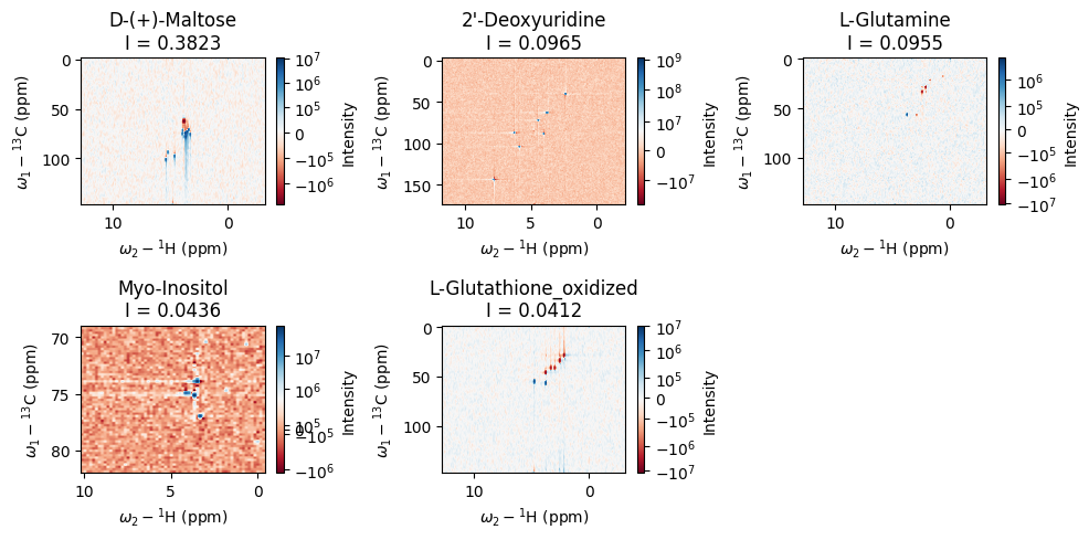
# Examine the main components spectra
_ = analyses[0].plot_top_spectra(k=5)
plt.tight_layout()

# Examine the residual to see what else needs to be explained
residual = analyses[0].build_residual()
residual.plot(absolute_values=True, cmap='Reds', backend='plotly')